Benchmarks

Tip

This page is a Jupyter notebook that can be downloaded and run locally. [1]

Adaptive sampling is a powerful technique for approximating functions with varying degrees of complexity across their domain. This approach is particularly useful for functions with sharp features or rapid changes, as it focuses on calculating more points around those areas. By concentrating points where they are needed most, adaptive sampling can provide an accurate representation of the function with fewer points compared to uniform sampling. This results in both faster convergence and a more accurate representation of the function.

On this benchmark showcase, we will explore the effectiveness of adaptive sampling for various 1D and 2D functions, including sharp peaks, Gaussian, sinusoidal, exponential decay, and Lorentzian functions. We will also present benchmarking results to highlight the advantages (and disadvantages) of adaptive sampling over uniform sampling in terms of an error ratio, which is the ratio of uniform error to learner error (see the note about the error below).

Look below where we demonstrate the use of the adaptive package to perform adaptive sampling and visualize the results. By the end of this benchmarking showcase, you should better understand of the benefits of adaptive sampling and in which cases you could to apply this technique to your own simulations or functions.

Note

Note on error estimates

The error is estimated using the L1 norm of the difference between the true function values and the interpolated values. Here’s a step-by-step explanation of how the error is calculated:

1. For each benchmark function, two learners are created: the adaptive learner and a homogeneous learner. The adaptive learner uses adaptive sampling, while the homogeneous learner uses a uniform grid of points.

2. After the adaptive learning is complete, the error is calculated by comparing the interpolated values obtained from the adaptive learner to the true function values evaluated at the points used by the homogeneous learner.

3. To calculate the error, the L1 norm is used. The L1 norm represents the average of the absolute differences between the true function values and the interpolated values. Specifically, it is calculated as the square root of the mean of the squared differences between the true function values and the interpolated values.

Note that the choice of the L1 norm is somewhat arbitrary. Please judge the results for yourself by looking at the plots and observe the significantly better function approximation obtained by the adaptive learner.

Warning

Note on benchmark functions

The benchmark functions used in this tutorial are analytical and cheap to evaluate. In real-world applications (see the gallery), adaptive sampling is often more beneficial for expensive simulations where function evaluations are computationally demanding or time-consuming.

Benchmarks 1D

Show code cell content Hide code cell content

from __future__ import annotations

import itertools

import holoviews as hv
import numpy as np
import pandas as pd
from scipy.interpolate import interp1d

import adaptive

adaptive.notebook_extension()

benchmarks = {}
benchmarks_2d = {}


def homogeneous_learner(learner):
    if isinstance(learner, adaptive.Learner1D):
        xs = np.linspace(*learner.bounds, learner.npoints)
        homo_learner = adaptive.Learner1D(learner.function, learner.bounds)
        homo_learner.tell_many(xs, learner.function(xs))
    else:
        homo_learner = adaptive.Learner2D(learner.function, bounds=learner.bounds)
        n = int(learner.npoints**0.5)
        xs, ys = (np.linspace(*bounds, n) for bounds in learner.bounds)
        xys = list(itertools.product(xs, ys))
        zs = map(homo_learner.function, xys)
        homo_learner.tell_many(xys, zs)
    return homo_learner


def plot(learner, other_learner):
    if isinstance(learner, adaptive.Learner1D):
        return learner.plot() + other_learner.plot()
    else:
        n = int(learner.npoints**0.5)
        return (
            (
                other_learner.plot(n).relabel("Homogeneous grid")
                + learner.plot().relabel("With adaptive")
                + other_learner.plot(n, tri_alpha=0.4)
                + learner.plot(tri_alpha=0.4)
            )
            .cols(2)
            .options(hv.opts.EdgePaths(color="w"))
        )


def err(ys, ys_other):
    abserr = np.abs(ys - ys_other)
    return np.average(abserr**2) ** 0.5


def l1_norm_error(learner, other_learner):
    if isinstance(learner, adaptive.Learner1D):
        ys_interp = interp1d(*learner.to_numpy().T)
        xs, _ = other_learner.to_numpy().T
        ys = ys_interp(xs)  # interpolate the other learner's points
        _, ys_other = other_learner.to_numpy().T
        return err(ys, ys_other)
    else:
        xys = other_learner.to_numpy()[:, :2]
        zs = learner.function(xys.T)
        interpolator = learner.interpolator()
        zs_interp = interpolator(xys)
        # Compute the L1 norm error between the true function and the interpolator
        return err(zs_interp, zs)


def run_and_plot(learner, **goal):
    adaptive.runner.simple(learner, **goal)
    homo_learner = homogeneous_learner(learner)
    bms = benchmarks if isinstance(learner, adaptive.Learner1D) else benchmarks_2d
    bm = {
        "npoints": learner.npoints,
        "error": l1_norm_error(learner, homo_learner),
        "uniform_error": l1_norm_error(homo_learner, learner),
    }
    bm["error_ratio"] = bm["uniform_error"] / bm["error"]
    bms[learner.function.__name__] = bm
    display(pd.DataFrame([bm]))  # noqa: F821
    return plot(learner, homo_learner).relabel(
        f"{learner.function.__name__} function with {learner.npoints} points"
    )


def to_df(benchmarks):
    df = pd.DataFrame(benchmarks).T
    df.sort_values("error_ratio", ascending=False, inplace=True)
    return df


def plot_benchmarks(df, max_ratio: float = 1000, *, log_scale: bool = True):
    import matplotlib.pyplot as plt
    import numpy as np

    df_hist = df.copy()

    # Replace infinite values with 1000
    df_hist.loc[np.isinf(df_hist.error_ratio), "error_ratio"] = max_ratio

    # Convert the DataFrame index (function names) into a column
    df_hist.reset_index(inplace=True)
    df_hist.rename(columns={"index": "function_name"}, inplace=True)

    # Create a list of colors based on the error_ratio values
    bar_colors = ["green" if x > 1 else "red" for x in df_hist["error_ratio"]]

    # Create the bar chart
    plt.figure(figsize=(12, 6))
    plt.bar(df_hist["function_name"], df_hist["error_ratio"], color=bar_colors)

    # Add a dashed horizontal line at 1
    plt.axhline(y=1, linestyle="--", color="gray", linewidth=1)

    if log_scale:
        # Set the y-axis to log scale
        plt.yscale("log")

    # Customize the plot
    plt.xlabel("Function Name")
    plt.ylabel("Error Ratio (uniform Error / Learner Error)")
    plt.title("Error Ratio Comparison for Different Functions")
    plt.xticks(rotation=45)

    # Show the plot
    plt.show()

1. Sharp peak function:

In the case of the sharp peak function, adaptive sampling performs very well because it can capture the peak by calculating more points around it, while still accurately representing the smoother regions of the function with fewer points.

def peak(x, offset=0.123):
    a = 0.01
    return x + a**2 / (a**2 + (x - offset) ** 2)


learner = adaptive.Learner1D(peak, bounds=(-1, 1))
run_and_plot(learner, loss_goal=0.1)

	npoints	error	uniform_error	error_ratio
0	34	0.004249	0.365365	85.98348

2. Gaussian function:

For smoother functions, like the Gaussian function, adaptive sampling may not provide a significant advantage over uniform sampling. Nonetheless, the algorithm still focuses on areas of the function that have more rapid changes, but the improvement over uniform sampling might be less noticeable.

def gaussian(x, mu=0, sigma=0.5):
    return (1 / np.sqrt(2 * np.pi * sigma**2)) * np.exp(
        -((x - mu) ** 2) / (2 * sigma**2)
    )


learner = adaptive.Learner1D(gaussian, bounds=(-5, 5))
run_and_plot(learner, loss_goal=0.1)

	npoints	error	uniform_error	error_ratio
0	39	0.003102	0.00759	2.446995

3. Sinusoidal function:

The sinusoidal function is another example of a smoother function where adaptive sampling doesn’t provide a substantial advantage over uniform sampling.

def sinusoidal(x, amplitude=1, frequency=1, phase=0):
    return amplitude * np.sin(frequency * x + phase)


learner = adaptive.Learner1D(sinusoidal, bounds=(-2 * np.pi, 2 * np.pi))
run_and_plot(learner, loss_goal=0.1)

	npoints	error	uniform_error	error_ratio
0	65	0.006611	0.000716	0.108295

4. Exponential decay function:

Adaptive sampling can be useful for the exponential decay function, as it focuses on the steeper part of the curve and allocates fewer points to the flatter region.

def exponential_decay(x, tau=1):
    return np.exp(-x / tau)


learner = adaptive.Learner1D(exponential_decay, bounds=(0, 5))
run_and_plot(learner, loss_goal=0.1)

	npoints	error	uniform_error	error_ratio
0	24	0.000825	0.001922	2.331293

5. Lorentzian function:

The Lorentzian function is another example of a function with a sharp peak. Adaptive sampling performs well in this case, as it concentrates points around the peak while calculating fewer points to the smoother regions of the function.

def lorentzian(x, x0=0, gamma=0.3):
    return (1 / np.pi) * (gamma / 2) / ((x - x0) ** 2 + (gamma / 2) ** 2)


learner = adaptive.Learner1D(lorentzian, bounds=(-5, 5))
run_and_plot(learner, loss_goal=0.1)

	npoints	error	uniform_error	error_ratio
0	43	0.005319	0.059005	11.093785

6. Sinc function:

The sinc function has oscillatory behavior with varying amplitude. Adaptive sampling is helpful in this case, as it can allocate more points around the oscillations, effectively capturing the shape of the function.

def sinc(x):
    return np.sinc(x / np.pi)


learner = adaptive.Learner1D(sinc, bounds=(-10, 10))
run_and_plot(learner, loss_goal=0.1)

	npoints	error	uniform_error	error_ratio
0	49	0.012649	0.002273	0.179731

7. Step function (Heaviside):

In the case of the step function, adaptive sampling efficiently allocates more points around the discontinuity, providing an accurate representation of the function.

import numpy as np


def step(x, x0=0):
    return np.heaviside(x - x0, 0.5)


learner = adaptive.Learner1D(step, bounds=(-5, 5))
run_and_plot(learner, npoints_goal=20)

/tmp/ipykernel_2972/4130640200.py:80: RuntimeWarning: divide by zero encountered in scalar divide
  bm["error_ratio"] = bm["uniform_error"] / bm["error"]

	npoints	error	uniform_error	error_ratio
0	20	0.0	0.260059	inf

8. Damped oscillation function:

The damped oscillation function has both oscillatory behavior and a decay component. Adaptive sampling can effectively capture the behavior of this function, calculating more points around the oscillations while using fewer points in the smoother regions.

def damped_oscillation(x, a=1, omega=1, gamma=0.1):
    return a * np.exp(-gamma * x) * np.sin(omega * x)


learner = adaptive.Learner1D(damped_oscillation, bounds=(-10, 10))
run_and_plot(learner, loss_goal=0.1)

	npoints	error	uniform_error	error_ratio
0	68	0.03329	0.007739	0.232478

9. Bump function (smooth function with compact support):

For the bump function, adaptive sampling concentrates points around the region of the bump, efficiently capturing its shape and calculating fewer points in the flatter regions.

def bump(x, a=1, x0=0, s=0.5):
    z = (x - x0) / s
    return np.where(np.abs(z) < 1, a * np.exp(-1 / (1 - z**2)), 0)


learner = adaptive.Learner1D(bump, bounds=(-5, 5))
run_and_plot(learner, loss_goal=0.1)

	npoints	error	uniform_error	error_ratio
0	47	0.000539	0.012031	22.299927

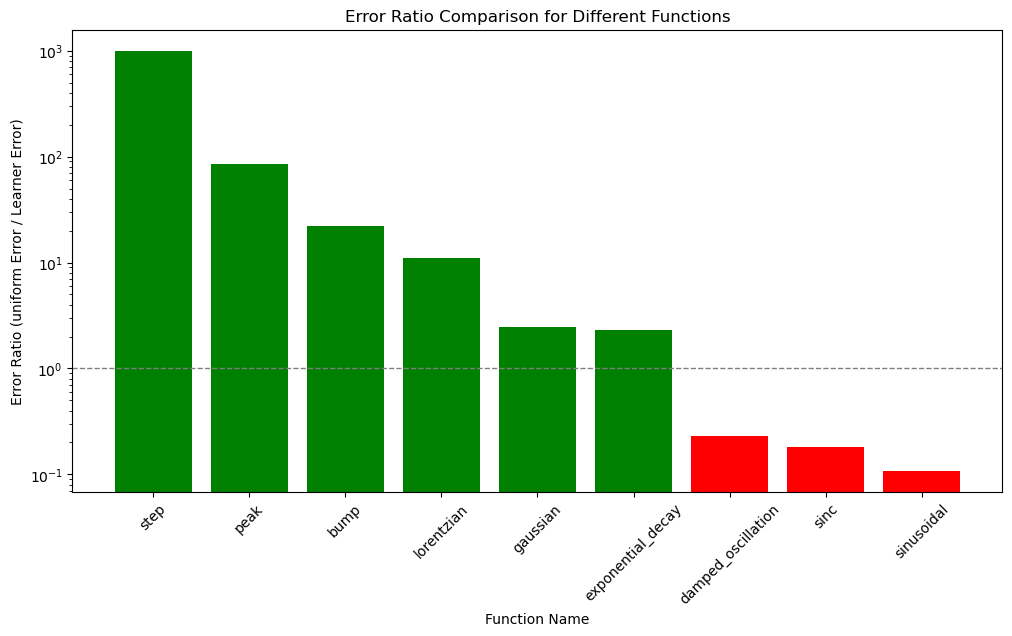
Results

In summary, adaptive sampling is a powerful approach for approximating functions with sharp features or varying degrees of complexity across their domain. It can efficiently allocate points where they are needed most, providing an accurate representation of the function while reducing the total number of points required. For smoother functions, adaptive sampling still focuses on areas with more rapid changes but may not provide significant advantages over uniform sampling.

df = to_df(benchmarks)
df

	npoints	error	uniform_error	error_ratio
step	20.0	0.000000	0.260059	inf
peak	34.0	0.004249	0.365365	85.983480
bump	47.0	0.000539	0.012031	22.299927
lorentzian	43.0	0.005319	0.059005	11.093785
gaussian	39.0	0.003102	0.007590	2.446995
exponential_decay	24.0	0.000825	0.001922	2.331293
damped_oscillation	68.0	0.033290	0.007739	0.232478
sinc	49.0	0.012649	0.002273	0.179731
sinusoidal	65.0	0.006611	0.000716	0.108295

plot_benchmarks(df)

Benchmarks 2D

1. Sharp ring:

This function has a ring structure in 2D.

def ring(xy, a=0.2):
    x, y = xy
    return x + np.exp(-((x**2 + y**2 - 0.75**2) ** 2) / a**4)


learner = adaptive.Learner2D(ring, bounds=[(-1, 1), (-1, 1)])
run_and_plot(learner, npoints_goal=1000)

	npoints	error	uniform_error	error_ratio
0	1000	0.886141	0.903228	1.019283

1. Gaussian surface: The Gaussian surface is a smooth, bell-shaped function in 2D. It has a peak at the mean (mu) and spreads out with increasing standard deviation (sigma). Adaptive sampling works well in this case because it can focus on the region around the peak where the function changes rapidly, while using fewer points in the flatter regions where the function changes slowly.

def gaussian_surface(xy, mu=(0, 0), sigma=(1, 1)):
    x, y = xy
    mu_x, mu_y = mu
    sigma_x, sigma_y = sigma
    return (1 / (2 * np.pi * sigma_x * sigma_y)) * np.exp(
        -((x - mu_x) ** 2 / (2 * sigma_x**2) + (y - mu_y) ** 2 / (2 * sigma_y**2))
    )


learner = adaptive.Learner2D(gaussian_surface, bounds=[(-5, 5), (-5, 5)])
run_and_plot(learner, loss_goal=0.01)

	npoints	error	uniform_error	error_ratio
0	170	0.03452	0.061862	1.792043

2. Sinusoidal surface: The sinusoidal surface is a product of two sinusoidal functions in the x and y directions. The surface has a regular pattern of peaks and valleys. Adaptive sampling works well in this case because it can adapt to the frequency of the sinusoidal pattern and allocate more points to areas with higher curvature, ensuring an accurate representation of the function.

def sinusoidal_surface(xy, amplitude=1, frequency=(0.3, 3)):
    x, y = xy
    freq_x, freq_y = frequency
    return amplitude * np.sin(freq_x * x) * np.sin(freq_y * y)


learner = adaptive.Learner2D(
    sinusoidal_surface, bounds=[(-2 * np.pi, 2 * np.pi), (-2 * np.pi, 2 * np.pi)]
)
run_and_plot(learner, loss_goal=0.01)

	npoints	error	uniform_error	error_ratio
0	1583	0.735665	0.882027	1.198953

def circular_peak(xy, x0=0, y0=0, a=0.01):
    x, y = xy
    r = np.sqrt((x - x0) ** 2 + (y - y0) ** 2)
    return r + a**2 / (a**2 + r**2)


learner = adaptive.Learner2D(circular_peak, bounds=[(-1, 1), (-1, 1)])
run_and_plot(learner, loss_goal=0.01)

	npoints	error	uniform_error	error_ratio
0	144	0.434798	0.462059	1.062699

4. Paraboloid:

The paraboloid is a smooth, curved surface defined by a quadratic function in the x and y directions. Adaptive sampling is less beneficial for this function compared to functions with sharp features, as the curvature is relatively constant across the entire surface. However, the adaptive algorithm can still provide a good representation of the paraboloid with fewer points than a uniform grid.

def paraboloid(xy, a=1, b=1):
    x, y = xy
    return a * x**2 + b * y**2


learner = adaptive.Learner2D(paraboloid, bounds=[(-5, 5), (-5, 5)])
run_and_plot(learner, loss_goal=0.01)

	npoints	error	uniform_error	error_ratio
0	158	17.442244	17.017536	0.975651

5. Cross-shaped function:

This function has a cross-shaped structure in 2D.

def cross(xy, a=0.2):
    x, y = xy
    return np.exp(-(x**2 + y**2) / a**2) * (
        np.cos(4 * np.pi * x) + np.cos(4 * np.pi * y)
    )


learner = adaptive.Learner2D(cross, bounds=[(-1, 1), (-1, 1)])
run_and_plot(learner, npoints_goal=1000)

	npoints	error	uniform_error	error_ratio
0	1000	0.205741	0.664969	3.232073

6. Mexican hat function (Ricker wavelet):

This function has a central peak surrounded by a circular trough.

def mexican_hat(xy, a=1):
    x, y = xy
    r2 = x**2 + y**2
    return a * (1 - r2) * np.exp(-r2 / 2)


learner = adaptive.Learner2D(mexican_hat, bounds=[(-2, 2), (-2, 2)])
run_and_plot(learner, npoints_goal=1000)

	npoints	error	uniform_error	error_ratio
0	1000	0.475294	0.582885	1.226368

7. Saddle surface:

This function has a saddle shape with increasing curvature along the diagonal.

def saddle(xy, a=1, b=1):
    x, y = xy
    return a * x**2 - b * y**2


learner = adaptive.Learner2D(saddle, bounds=[(-2, 2), (-2, 2)])
run_and_plot(learner, npoints_goal=1000)

	npoints	error	uniform_error	error_ratio
0	1000	2.538706	2.54007	1.000537

8. Steep linear ramp:

This function has a steep linear ramp in a narrow region.

def steep_ramp(xy, width=0.1):
    x, y = xy
    result = np.where((-width / 2 < x) & (x < width / 2), 10 * x + y, y)
    return result


learner = adaptive.Learner2D(steep_ramp, bounds=[(-1, 1), (-1, 1)])
run_and_plot(learner, loss_goal=0.005)

	npoints	error	uniform_error	error_ratio
0	634	0.84986	0.884934	1.041271

9. Localized sharp peak:

This function has a sharp peak in a small localized area.

def localized_sharp_peak(xy, x0=0, y0=0, a=0.01):
    x, y = xy
    r = np.sqrt((x - x0) ** 2 + (y - y0) ** 2)
    return r + a**4 / (a**4 + r**4)


learner = adaptive.Learner2D(localized_sharp_peak, bounds=[(-1, 1), (-1, 1)])
run_and_plot(learner, loss_goal=0.01)

	npoints	error	uniform_error	error_ratio
0	143	0.433102	0.459874	1.061815

10. Ridge function:

A function with a narrow ridge along the x-axis, which can be controlled by a parameter b.

def ridge_function(xy, b=100):
    x, y = xy
    return np.exp(-b * y**2) * np.sin(x)


learner = adaptive.Learner2D(ridge_function, bounds=[(-2, 2), (-1, 1)])
run_and_plot(learner, loss_goal=0.01)

	npoints	error	uniform_error	error_ratio
0	248	0.287239	0.57165	1.990154

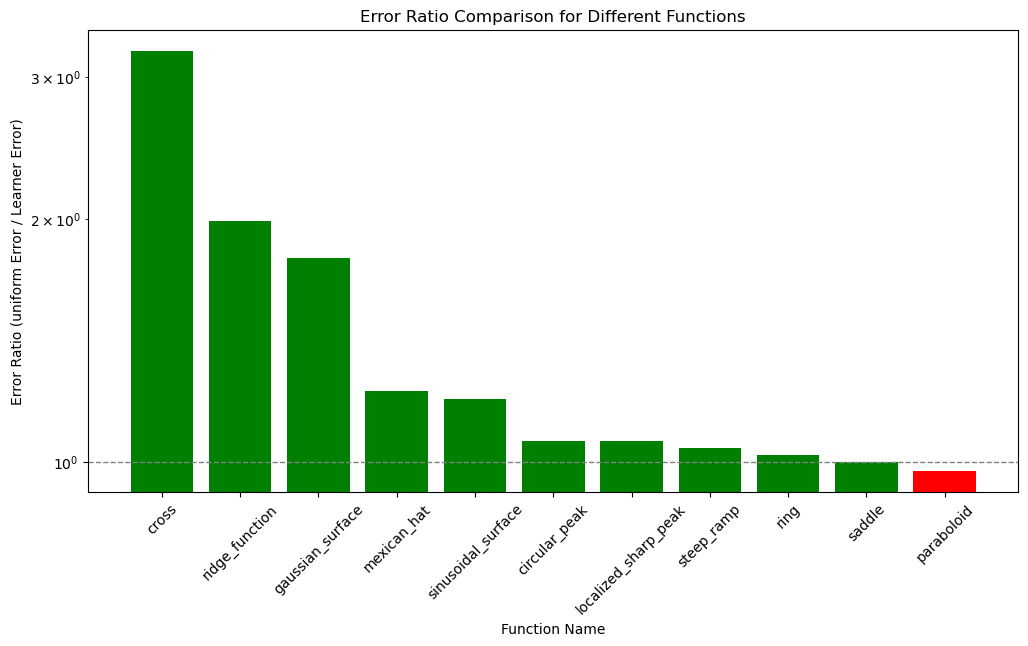
Results

df = to_df(benchmarks_2d)
df[["npoints", "error_ratio"]]

	npoints	error_ratio
cross	1000.0	3.232073
ridge_function	248.0	1.990154
gaussian_surface	170.0	1.792043
mexican_hat	1000.0	1.226368
sinusoidal_surface	1583.0	1.198953
circular_peak	144.0	1.062699
localized_sharp_peak	143.0	1.061815
steep_ramp	634.0	1.041271
ring	1000.0	1.019283
saddle	1000.0	1.000537
paraboloid	158.0	0.975651

plot_benchmarks(df)

---

[1]

This notebook can be downloaded as benchmarks.ipynb and benchmarks.md.